Solid Extrusions
A classic way for generating 3d solids is the application of a virtual extrusion operation. For this, one needs a basic sketch and calls the extrusion function.
In its most simple form, the extrusion() function takes just the sketch as a first argument and a spanning vector as a second argument. The spanning vector should purlely lie on the X/Y plane since it defines in which direction the sketch gets extruded. In the following example, we assume the sketch to be the one used in the section about sketches:
Example
make extrusion( s, <[0,0,1]> )

Extrusion of the smiley contour.
Winding number mechanism
Now how does it come that some areas of the smiley sketch are actually solid while others are empty? Remembering the four different curves that were involved in the sketch definition, one can see that every curve has its own loop orientation. These orientations allows the calculation of a winding number for every partial area of the sketch. This allows to determine the resulting state of each area: if its winding number is zero, the area will be empty, otherwise it will be solid.
The usage of winding number is especially interesting for sketches with overlapping curves. The following example shows this for three overlapping curves:
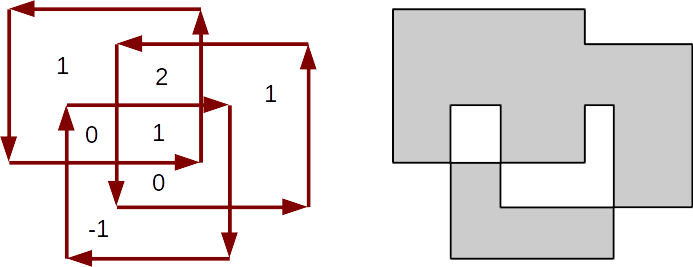
Three overlapping curves with winding numbers (left) and the resulting areas (right).
Extrusions along paths
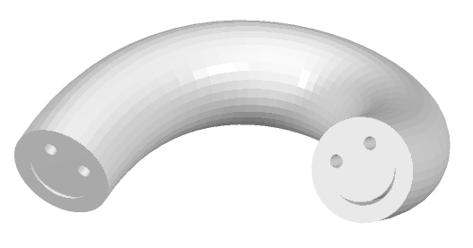
Extrusions do not necessarily need to be applied along a span vector only: instead they can be applied along a curve that acts as an extrusion path. This allows to "build" elements like bars, pipes and many others. An extrusion along a path is shown in the following example:
Example
curve p = <[0,0]> -> bezier( <[50,0]>, <[50,-20,50]>, <[0,20,50]> )
make extrusion( s, p )
Apart from that, extrusions have a number of additional options. For more information see the reference page.